You know that predictive design that you spent HOURS working on…what would you say if I told you that it is wrong before you ever added the first simulated AP? Are you in shock? Don’t be. It’s not your fault.

I recently took part in an intriguing conversation about Ekahau predictive designs. The crux of the discussion was whether or not the AP output power shown in the predictive survey is the same power level (assuming no impediments existed) as what exists in a real world deployment. Did you know that for data transmissions the answer is no? Let’s take a look at a reason why.

Don’t worry, I’m not going to make you read all the way to the end. Let’s just get this over with now.

The EIRP value shown by Ekahau for a given radio does not take into account MIMO gains when calculating predictive coverage.

When Ekahau performs the calculations to determine coverage levels within your project, it uses EIRP of the AP along with things like Free Space Path Loss (FSPL) and wall attenuation values to run the numbers. The problem is that the peak EIRP value can change based upon the number of radio chains in the AP. You’ll notice in my previous post Aruba lists EIRP with the peak antenna gain, and a peak antenna gain calculated with the combined average of all of the antenna elements for a given radio/band. Onno Harms, of Aruba, describes this more in detail here:

Traditionally, peak EIRP would be calculated by adding the peak antenna gain to the max conducted power and multiply this by the number of radio chains (equivalent to adding 6dB for a 4×4 radio, or 3dB for a 2×2 radio). This is ok if the conducted power is the same for all radio chains (typically true) and if the peaks for all patterns line up perfectly (in a 3D space). That is generally not the case, and in reality the peak EIRP is significantly lower.

Source: Aruba Airheads Community, Onno Harms, Aruba – https://community.arubanetworks.com/t5/Wireless-Access/Antenna-gain-with-MIMO/td-p/488196

The formula to calculate EIRP is:

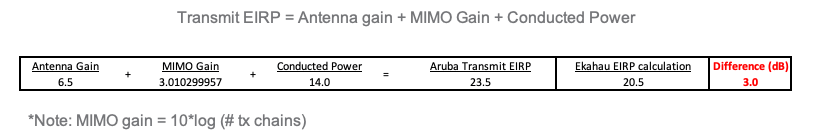
Transmit EIRP = Antenna gain + MIMO Gain + Conducted Power – system loss (connectors, cables, etc)

This is important to note as the power output calculated by Ekahau will actually be LESS than what it is in a real world scenario when the AP is Tx to the client (which is what Ekahau is modeling). OK so that sounds scary, but is the differential really that much that I should be concerned?

In order to calculate the EIRP from an AP, you’ll need to gather a couple of pieces of information. First, from the AP datasheet you will need to find the value of the antenna gain (see my previous post on which value to use if more than one). You will also need to know what the MIMO gain of the AP is. TIP: MIMO gain is calculated as 10 * log (# of tx chains) in case you didn’t have that handy. 🙂

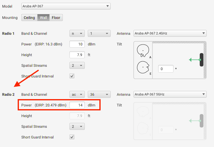
If you look at the following calculation, you will see that with a conducted (transmit) power of 14 dBm, the actual Aruba EIRP is 23.5 dBm (note: we’re assuming negligible loss with an integrated antenna system), yet the Ekahau calculation (shown in Radio 2 Ekahau example image above) is only 20.5 dBm. That’s a difference of 3 dB which means Ekahau is modeling half the power that is actually being output by the system!

How can you validate this? If you have an Aruba system, you can find the conducted power of the radio by using the following command on your Aruba controller.

aruba# show ap debug power-table ap-name <ap-name> radio <radio #>

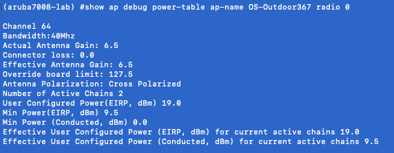
As you can see in the CLI output above, the next to last line shows the Effective User Configured Power (EIRP, dBm). If you use the formula above you can see how the math works out.

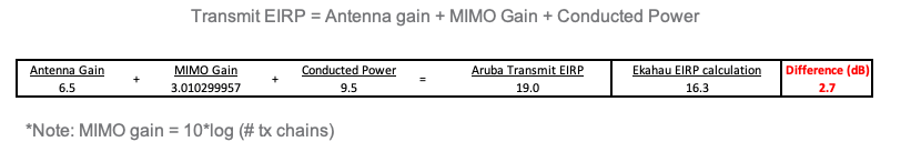
You can look at Radio 1 in the Ekahau AP Radio Settings image above and see that with a Tx power of 9.5 dBm (Ekahau rounds to 10 dBm), and an antenna gain of 6.5 dBi, Ekahau determines the EIRP to be 16.3 dBm when in reality it is 19 dBm.

So back to the question of is this something to really worry about? Possibly. The 3dB differential I show above is only what exists from a 2×2 radio. Now that we are seeing mostly 4×4 radios deployed (and soon 8×8) the differential jumps to 6 dB and 9 dB, respectively. While 3dB may fall within a statistical category of insignificance to you, 6 and 9 dB start to get pretty high and should be taken into consideration.

Keep in mind this discussion has focused on the environment only from the side of the AP, and this variation applies to all frames regardless of what data rate the frame is sent at! Head spinning? Already questioning if predictive designs are worth the trouble? We haven’t made it to the way the client sees the world yet, which opens a whole new can of worms! If you’re wondering if I’m trying to tell you that predictive designs are not worth it, I’m NOT saying that at all.

Let’s be clear on that. Tools such as Ekahau, iBwave, etc can’t take into account every single thing that could cause the signal level to fluctuate. These tools are the best we have for now and with the variability of client receive sensitivity, I’m not sure we could ever model these things with a high degree of accuracy. Predictive designs are BEST EFFORT. Any good Wi-Fi engineer will tell you, don’t just rely on the predictive. Go out and test YOUR environment, with YOUR devices, and adjust accordingly.

Just something to keep in mind when working with your Ekahau predictive designs. MIMO gains matter!

-Scott

*Some images courtesy of Aruba Networks